[Kaggle] Spaceship Titanic Competition

[Kaggle] Space Ship Titanic 생존자 예측
Welcome to the year 2912, where your data science skills are needed to solve a cosmic mystery. We’ve received a transmission from four lightyears away and things aren’t looking good.
The Spaceship Titanic was an interstellar passenger liner launched a month ago. With almost 13,000 passengers on board, the vessel set out on its maiden voyage transporting emigrants from our solar system to three newly habitable exoplanets orbiting nearby stars.
While rounding Alpha Centauri en route to its first destination—the torrid 55 Cancri E—the unwary Spaceship Titanic collided with a spacetime anomaly hidden within a dust cloud. Sadly, it met a similar fate as its namesake from 1000 years before. Though the ship stayed intact, almost half of the passengers were transported to an alternate dimension!
Titanic 생존자 예측과 비슷한 문제로 우주선 탑승객이 다른 차원으로 이동 되었는지 아닌지 예측하는 모델을 만드는 문제입니다.
1. Checking Data
Data Columns
PassingerId- 승객의 고유 ID, gggg_pp 형태이며, gggg는 여행자 그룹을 나타내고 pp는 그룹 내에서 자신의 번호를 나타냄.HomePlanet- 승객의 출발 행성
CryoSleep- 항해 중 승객의 동면 여부Cabin- 승객의 객실 번호 deck/num/side의 형태를 취하며 side의 경우 Port(좌현)과 Starboard(우현)으로 나뉨
Destination- 승객의 목적지를 나타냄Age- 승객의 나이VIP- 승객이 항해 중 특별 VIP 서비스 비용을 지불했는지 여부RoomService,FoodCourt,ShoppingMall,Spa,VRDeck- 승객이 여러 고급 편의 시설에서 청구한 금액
Name- 승객의 이름
Transported- 승객이 다른 차원으로 이동 되었는지 여부 (Target Data)
Note
PassingerId의 경우 승객 고유의 값이기 때문에 직접적으로 학습에 활용하기에는 무리가 있으나 그룹 정보를 포함하고 있기 때문에 잘 정제해서 같은 그룹에 포함된 인원의 수와 같은 데이터로 가공한다면 활용 가능할 것이라고 생각하였습니다.Cabin의 경우 3개의 Featuredeck,num,side가 합쳐진 형태이므로 일단 분리해서 3개의 Columns으로 만들어 활용하는 것이 좋을 것 같습니다.
Import Packages
1
2
3
4
5
6
7
8
9
10
11
12
13
14
15
16
17
18
19
20
21
22
23
24
import numpy as np # linear algebra
import pandas as pd # data processing, CSV file I/O (e.g. pd.read_csv)
from sklearn.preprocessing import LabelEncoder
import xgboost as xgb
from sklearn.model_selection import train_test_split
from sklearn.metrics import balanced_accuracy_score
from sklearn.model_selection import GridSearchCV

%matplotlib inline

import matplotlib.pyplot as plt
import seaborn as sns

plt.style.use('seaborn')
sns.set(font_scale=2)

import warnings

warnings.filterwarnings('ignore')

import os
for dirname, _, filenames in os.walk('/kaggle/input'):
    for filename in filenames:
        print(os.path.join(dirname, filename))
Load Dataset
1
2
train_df = pd.read_csv("/kaggle/input/spaceship-titanic/train.csv")
test_df = pd.read_csv("/kaggle/input/spaceship-titanic/test.csv")
2. Feature Engineering
Split Cabin
Cabin을 ‘/’를 기준으로 나눠서 deck, num, side 3개의 Feature로 분할
1
2
train_df[['Deck', 'Num', 'Side']] = train_df['Cabin'].str.split('/', expand=True) # Separate cabin data in deck, num, and side
test_df[['Deck', 'Num', 'Side']] = test_df['Cabin'].str.split('/', expand=True)
Count Group and Create New Feature
PassingerId를 Group과 PassengerNum 두 개의 Feature로 분할
1
2
train_df[['Group', 'PassengerNum']] = train_df['PassengerId'].str.split('_', expand=True) # Separate cabin data in deck, num, and side
test_df[['Group', 'PassengerNum']] = test_df['PassengerId'].str.split('_', expand=True)
Group Column에서 각각의 그룹의 수를 세서 새로운 Group_size Feature을 생성
1
2
train_df['Group_size'] = train_df['Group'].map(lambda x: pd.concat([train_df['Group'], test_df['Group']]).value_counts()[x])
test_df['Group_size'] = test_df['Group'].map(lambda x: pd.concat([train_df['Group'], test_df['Group']]).value_counts()[x])
Drop Unwanted Columns
1
2
train_df.drop(['PassengerId', 'Name', 'Cabin', 'Group', 'PassengerNum'],axis=1,inplace=True)
test_df.drop(['Name', 'Cabin', 'Group', 'PassengerNum'],axis=1,inplace=True)
Handling Missing Value
결측치는 중앙값과 최빈값으로 채우겠습니다.
1
train_df.isnull().sum()
1
2
3
4
5
6
7
8
9
10
11
for col in train_df.select_dtypes('object').columns: # Replace NaN values in Norminal data columns with mode value
    train_df[col] = train_df[col].fillna(train_df[col].mode()[0])

for col in train_df.select_dtypes('number').columns: # Replace NaN values in Norminal data columns with mode value
    train_df[col] = train_df[col].fillna(train_df[col].median())

for col in test_df.select_dtypes('object').columns: # Replace NaN values in Norminal data columns with mode value
    test_df[col] = test_df[col].fillna(test_df[col].mode()[0])

for col in test_df.select_dtypes('number').columns: # Replace NaN values in Norminal data columns with mode value
    test_df[col] = test_df[col].fillna(test_df[col].mode()[0])
3. EDA
1. Transported (Target)
1
2
3
4
5
6
7
fig, ax = plt.subplots(1, 2, figsize=(14,5))

train_df['Transported'].value_counts().plot.pie(ax=ax[0], explode=[0,0.1], shadow=True, autopct='%1.1f%%', labels=labels)

sns.countplot(data=train_df, x='Transported', ax=ax[1])

plt.show()
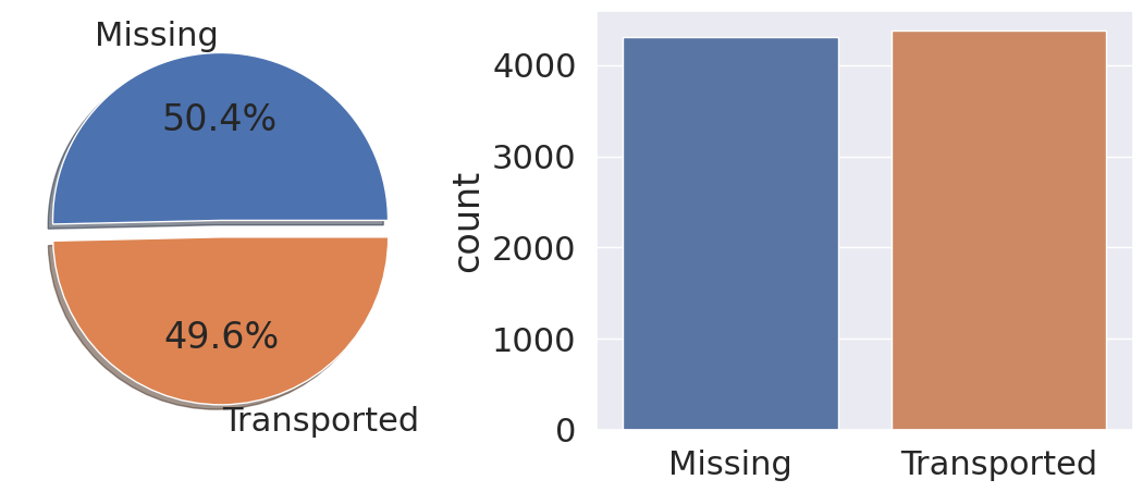
항해 중 다른 차원으로 이동 된 사람들과 그렇지 않은 사람들의 비율이 비슷하기 때문에 데이터의 샘플링은 불필요 할 것 같습니다.
2. HomePlanet
1
2
3
4
5
fig, ax = plt.subplots(figsize=(6,6))

sns.countplot(data=train_df, x='HomePlanet', hue='Transported', ax=ax)

plt.show()
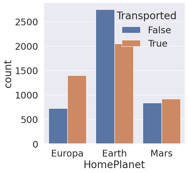
1
train_df[['HomePlanet', 'Transported']].groupby(['HomePlanet'], as_index=False).mean().sort_values(by='Transported', ascending=False)
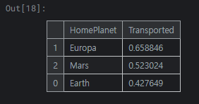
지구, 유로파, 화성 순으로 탑승 승객이 많으며, 지구에서 탑승한 승객들이 다른 두 행성에서 탑승한 승객들보다 이동 확률이 낮음을 확인 가능합니다.
3. CryoSleep
1
2
3
4
5
fig, ax = plt.subplots(figsize=(6,6))

sns.countplot(data=train_df, x='CryoSleep', hue='Transported', ax=ax)

plt.show()
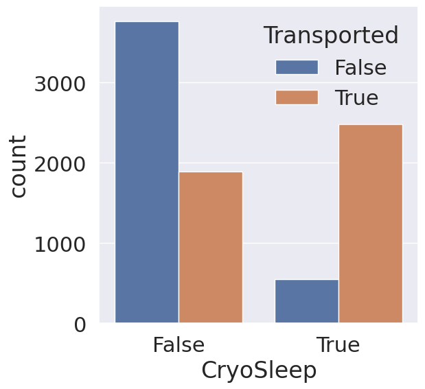
CryoSleep의 경우 동면 중인 승객들이 그렇지 않은 승객들에 비해 이동 확률이 높은 것을 확인 가능합니다. CryoSleep은 학습에 유의미하게 사용할 수 있겠습니다.
4. Cabin (Deck)
1
2
3
4
5
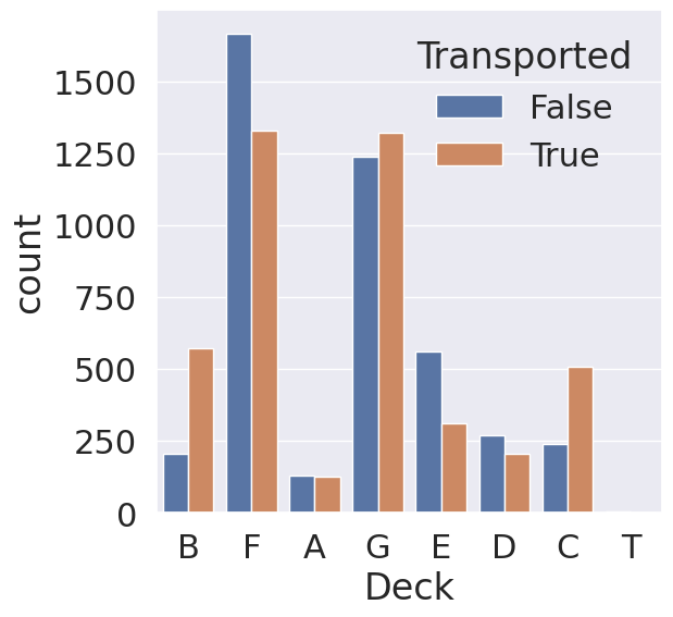
fig, ax = plt.subplots(figsize=(6,6))
sns.countplot(data=train_df, x='Deck', hue='Transported', ax=ax)
plt.show()
1
train_df[['Deck', 'Transported']].groupby(['Deck'], as_index=False).mean().sort_values(by='Transported', ascending=False)
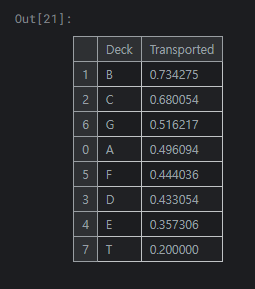
각 Cabin에서 승객이 제대로 도착한 비율을 구해보면 다음과 같습니다. 객실 B와 C의 경우 승객의 이동 확률에 유의미한 차이가 있음을 확인 가능합니다.
5. Cabin (Side)
1
2
3
4
5
fig, ax = plt.subplots(figsize=(6,6))

sns.countplot(data=train_df, x='Side', hue='Transported', ax=ax)

plt.show()

1
train_df[['Side', 'Transported']].groupby(['Side'], as_index=False).mean().sort_values(by='Transported', ascending=False)
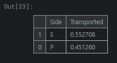
Side의 경우 우현(S)에 앉은 승객들이 좌현(P)에 앉은 승객들보다 이동 확률이 높다는 것을 확인 가능합니다.
6. Destination
1
2
3
4
5
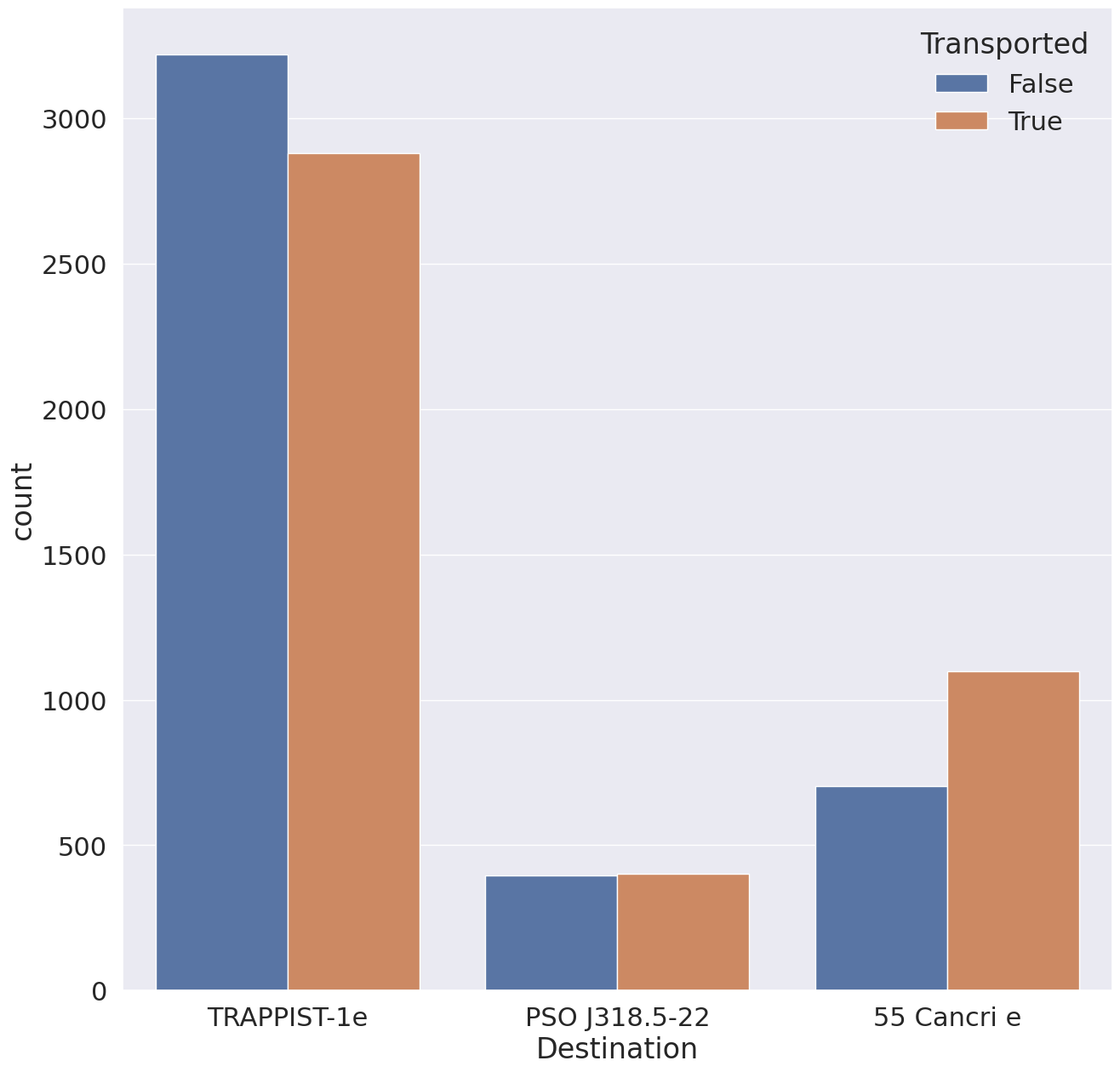
fig, ax = plt.subplots(figsize=(15,15))
sns.countplot(data=train_df, x='Destination', hue='Transported', ax=ax)
plt.show()
1
train_df[['Destination', 'Transported']].groupby(['Destination'], as_index=False).mean().sort_values(by='Transported', ascending=False)
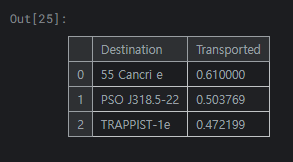
55 Cancri e가 목적지였던 승객들은 이동 확률이 높고 TRAPPIST-1e가 목적지인 승객은 이동 확률이 낮음을 확인 가능합니다.
7. Age
1
2
3
4
5
6
fig, ax = plt.subplots(1, 1, figsize=(9, 5))
sns.kdeplot(train_df[train_df['Transported'] == False]['Age'], ax=ax)
sns.kdeplot(train_df[train_df['Transported'] == True]['Age'], ax=ax)
lable = ['False', 'True']
plt.legend(labels=lable)
plt.show()
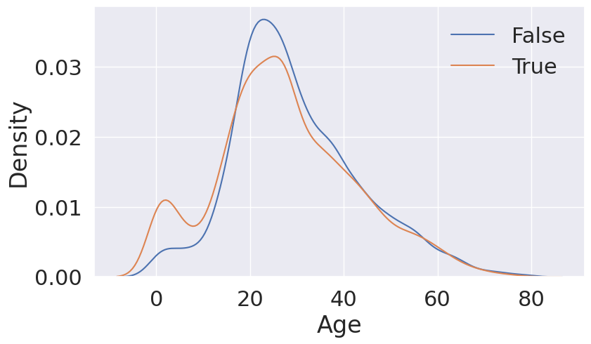
0 ~ 18세까지는 이동 확률이 높으며, 19 ~ 40세까지는 이동 확률이 낮은 것을 확인 가능합니다.
8. VIP
1
2
3
4
5
fig, ax = plt.subplots(figsize=(6,6))

sns.countplot(data=train_df, x='Side', hue='Transported', ax=ax)

plt.show()
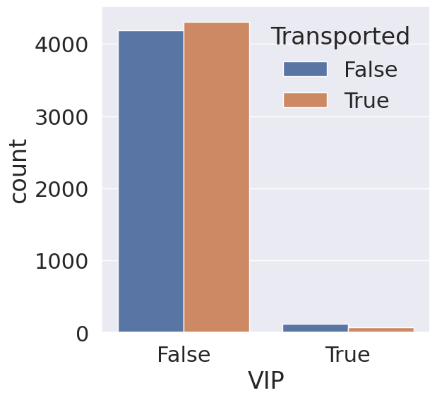
VIP의 경우 신청한 승객과 그렇지 않은 승객들 간의 이동 확률의 차이가 거의 없음을 확인할 수 있으며, 학습에 큰 영향을 주지 못할 것 같습니다.
9. RoomService, FoodCourt, ShoppingMall, Spa, VRDeck
1
2
3
4
5
6
7
8
9
10
fig, ax = plt.subplots(5, 1, figsize=(10, 20))
fig.subplots_adjust(hspace=0.6,wspace=0.6)
sns.set(font_scale=1.5)

num_list = ['RoomService', 'FoodCourt', 'ShoppingMall', 'Spa', 'VRDeck']

for i, columns in enumerate(num_list):
    sns.histplot(data=train_df, x=columns, ax=ax[i], bins=30, kde=False, hue='Transported')

plt.show()
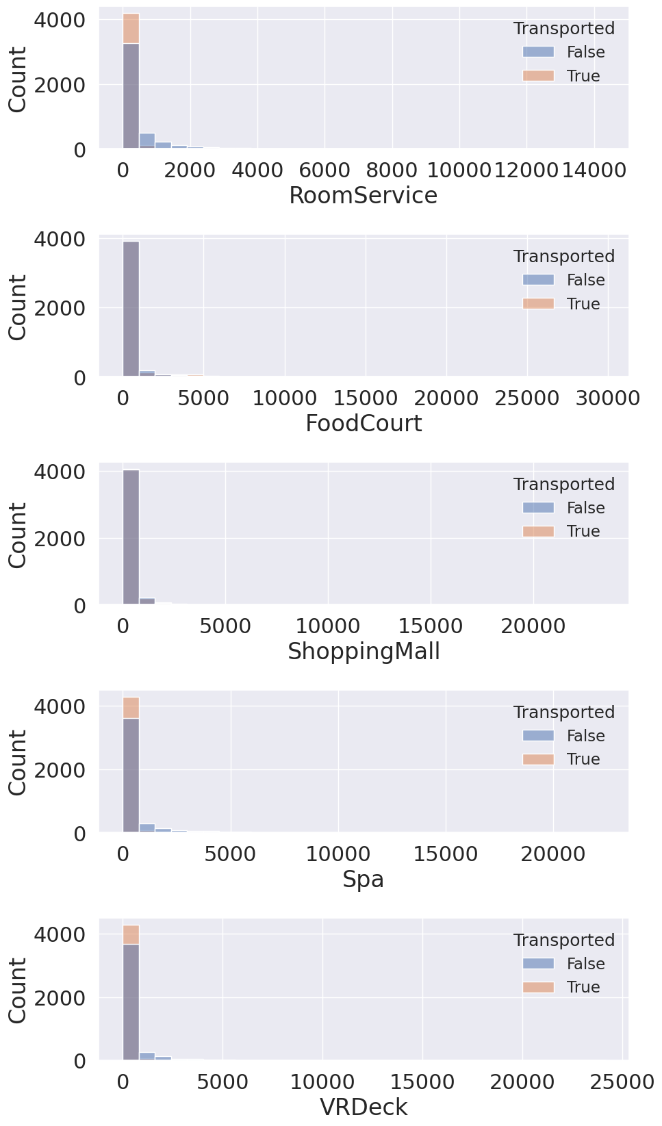
위 데이터들은 특이하게도 대부분이 0이며, 이는 소수의 승객들만이 유료 서비스를 이용했음을 나타냅니다. 그래프로 출력해 보았을 때 데이터 분포의 첨도가 매우 높음을 확인 가능합니다.
10. Correlation matrix
1
2
3
plt.figure(figsize=(15,15))
sns.heatmap(train_df.corr( ) , cmap='coolwarm', annot=True, fmt = '.2f')
plt.show( )
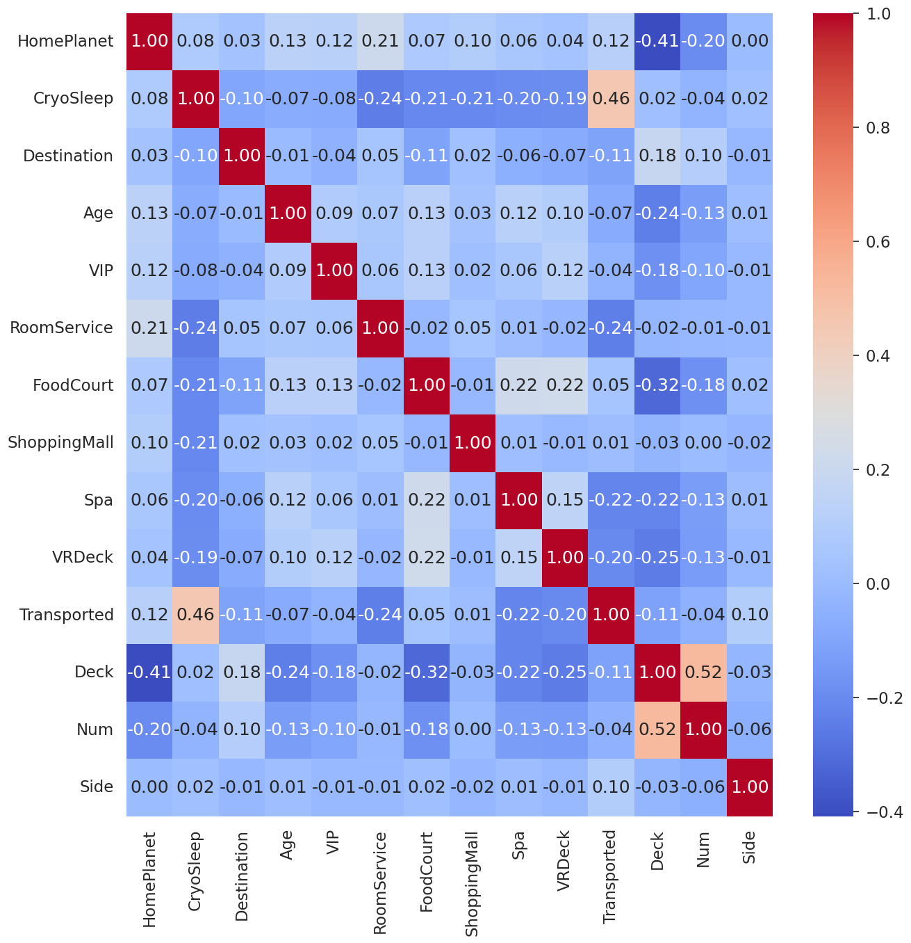
CryoSleep이 Target과 강한 상관 관계를 가지고 있음을 확인 가능합니다.
4. Preprocessing
1. Integer conversion
1
2
3
4
5
int_list = ['CryoSleep', 'VIP', 'Num']

for i in int_list:
    train_df[i] = train_df[i].astype('int')
    test_df[i] = test_df[i].astype('int')
bool 자료형 또는 숫자로 이루어져 있지만 현재 문자 형인 변수를 Int 자료형으로 변환
2. Label Encoding
1
2
3
4
5
6
7
8
9
10
11
12
13
14
label_list = ['HomePlanet', 'Destination', 'Deck', 'Num', 'Side']

for i in label_list:
    le = LabelEncoder()

    le = le.fit(train_df[i])

    train_df[i] = le.transform(train_df[i])

    for label in test_df[i]:
        if label not in le.classes_:
            le.classes_ = np.append(le.classes_,label)

    test_df[i] = le.transform(test_df[i])
모델이 인식할 수 있도록 object 형태의 Feature 들을 정수의 형태로 Label encoding
3. Split Train & Test Data
1
2
3
4
X = train_df.drop('Transported', axis=1).copy()
Y = train_df['Transported'].copy()

X_train, X_test, Y_train, Y_test = train_test_split(X, Y, random_state=42)
5. Modelling
1. First Training with XGBoost
1
2
3
4
5
6
7
8
9
clf_xgb = xgb.XGBClassifier(object='binary:logistic', missing=None)
clf_xgb.fit(
    X_train,
    Y_train,
    verbose=True,
    early_stopping_rounds=10,
    eval_metric='aucpr',
    eval_set=[(X_test,Y_test)]
)
Validation Accuracy: 0.90573
2. Hyperparameter optimization Using GridSearchCV
1
2
3
4
5
6
7
8
9
10
11
12
13
14
15
16
17
18
19
20
param_grid={
    'max_depth': [3,4,5],
    'learning_rate': [1, 0.5, 0.1, 0.01, 0.05],
    'gamma': [0, 0.25, 1.0],
    'reg_lambda': [0, 1.0, 10.0, 20, 100],
    'scale_pos_weght': [1, 3, 5]
}

optimal_params = GridSearchCV(
    estimator=xgb.XGBClassifier(
        object='binary:logistic',
        subsample=0.9,
        colsample_bytree=0.5
    ),
    param_grid=param_grid,
    scoring='roc_auc',
    verbose=0,
    n_jobs=10,
    cv=3
)
3. Second Training
1
2
3
4
5
6
7
8
9
10
11
12
13
14
15
16
17
18
clf_xgb = xgb.XGBClassifier(object='binary:logistic',
                            gamma=0.25,
                            learning_rate=0.1,
                            max_depth=4,
                            reg_lambda=10,
                            scale_pos_weght=3,
                            subsample=0.9,
                            colsample_bytree=0.5
                           )

clf_xgb.fit(
    X_train,
    Y_train,
    verbose=True,
    early_stopping_rounds=10,
    eval_metric='aucpr',
    eval_set=[(X_test,Y_test)]
)
Validation Accuracy: 0.90642
6. Review
첫 Competitions이라 아직 EDA가 미숙해 데이터의 특성을 파악해도 어떤 가공을 해야 하는지 어떤 데이터를 drop 해야 하는지 어려웠지만 그만큼 배운 것도 많은 것 같습니다.
Submit 점수는 처음엔 낮았지만 PassingerId를 정제하여 Group_size를 새로 만드는 등의 수정을 통해서 점수가 많이 상승했습니다.
이번 Competitions 통해서 제대로 된 Feature Engineering의 중요성을 확인한 것 같습니다!